This test determines the position error of each collimator leaf at a variety of positions. For each leaf position, the expected (from RTPLAN with collimator center position added) position is subtracted from the measured position and the error reported in mm in the isoplane:
error = measured - expected
The first step in the analysis is to measure the positions of the leaf sides. Accurate measurements are necessary to isolate the positions of a leaf end from the adjacent leaves.
The following example from a Millenium collimator shows the measured positions of the leaf ends and sides (as dashed lines) as well as the expected (planned) positions, compensated with the results from the collimator centering, shown as solid lines.
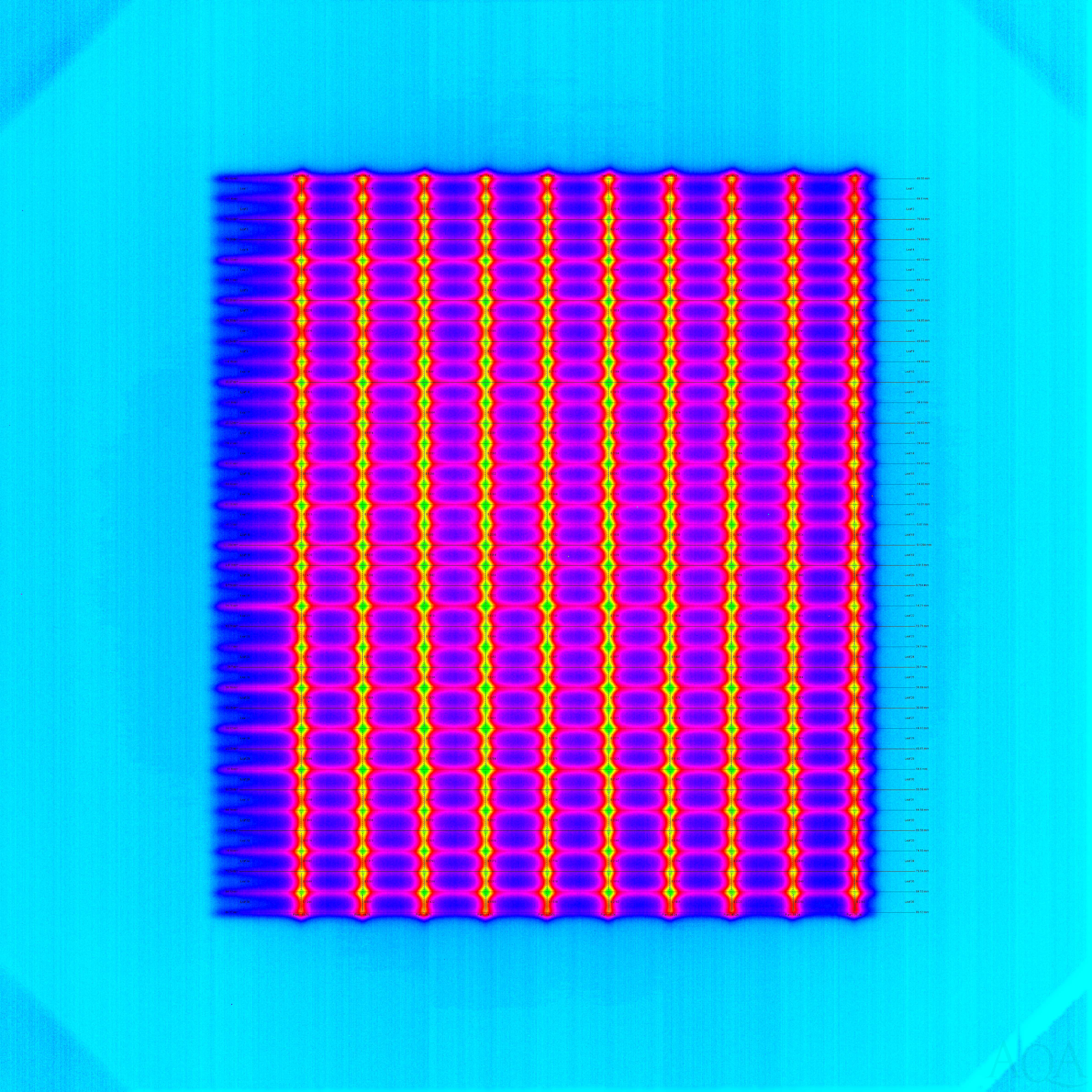
To measure the leaf sides, the sum of each row (or columns if the collimator were turned 90 degrees) of pixels in the entire image is taken, which yields a profile. The following graph shows an example taken from a Millenium collimator showing a peak for each leaf side (click for full size image):
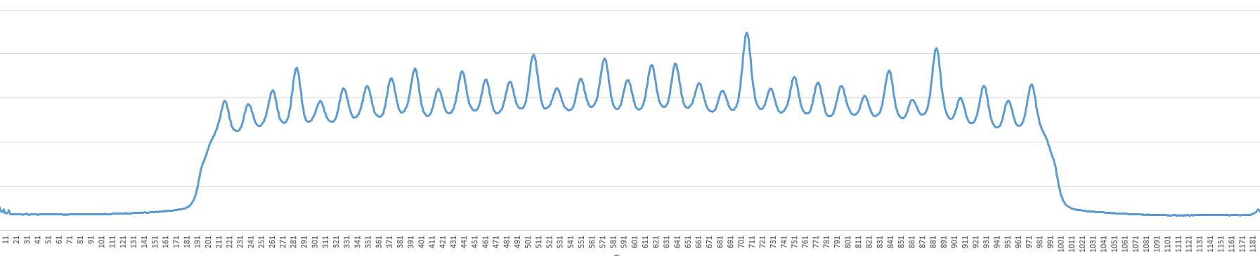
Using the expected widths of the leaves, the profile is traversed to obtain a rough estimate of the difference in height between the peaks and valleys. A qualitative measurement is made for each peak. A well defined peak is one that shows an adjacent valley at the expected distance on either side.
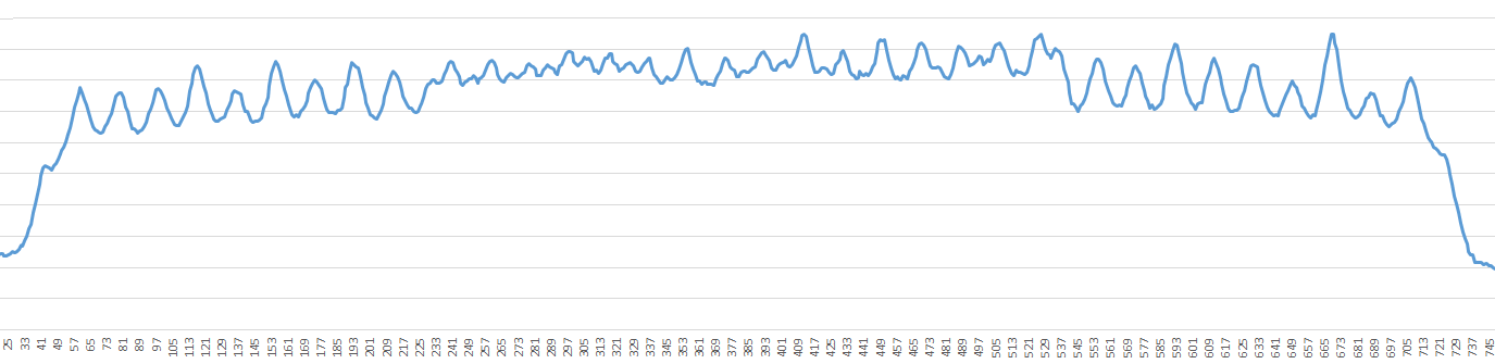
While the above profile shows well-defined peaks and valleys, images from HD MLC collimators can be less so. Below is an example of the image from an HD MLC collimator followed by a leaf-side profile for an HD MLC collimator:
An example from an HD MLC collimator (click for full size image):
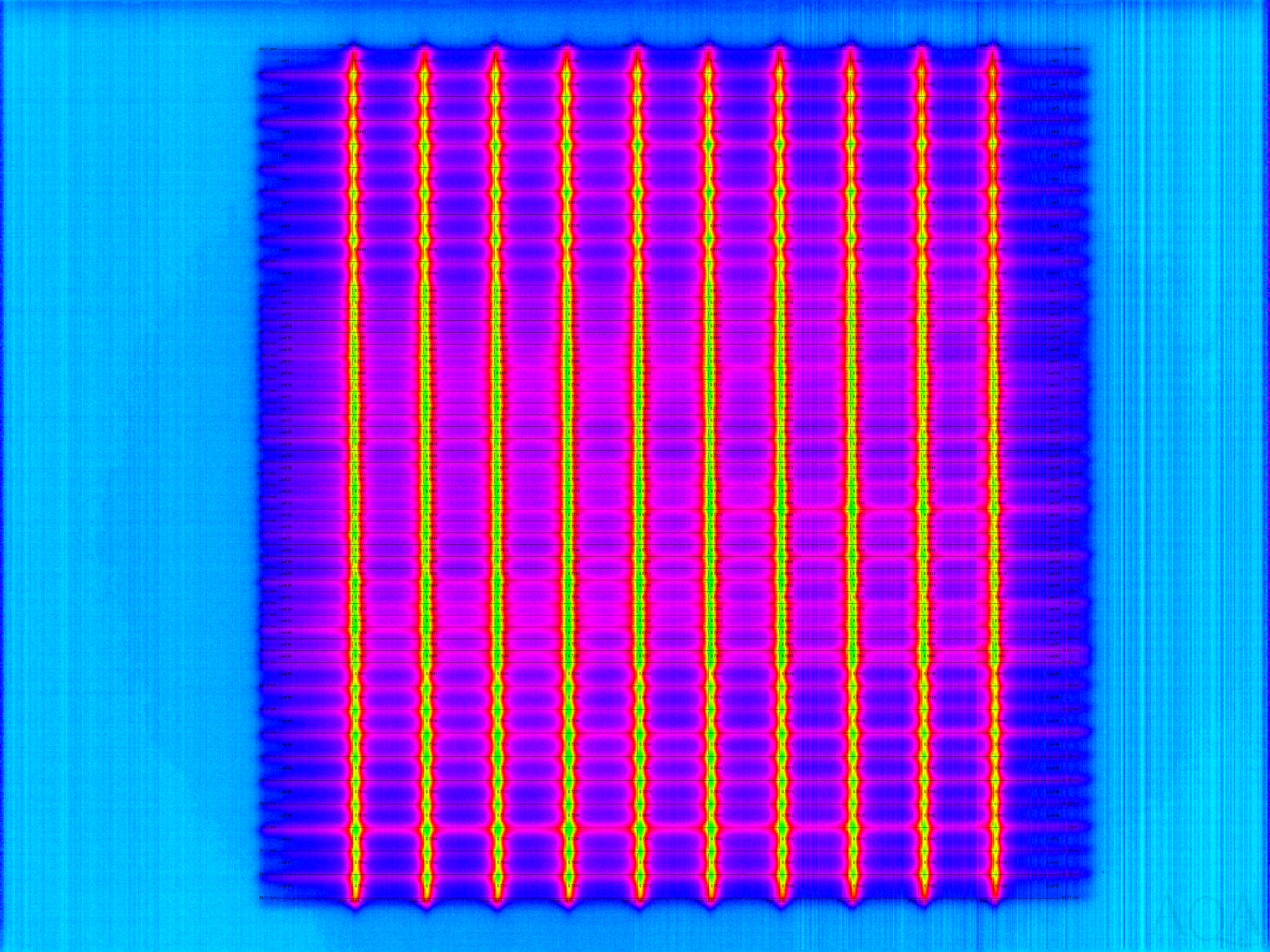
Because the positions of some leaf sides can be difficult to discriminate, only the best (in terms of peak-valley rise and fall) defined leaf sides are used. The assumption is made that at least two leaf sides will be well defined.
Given the best defined leaf sides, a cubic spline is mathematically calculated over the peaks using the profile. The resulting cubic spline function is searched for the highest point, which is the exact position of the peak.
The exact peak positions are matched with their nearest expected leaf sides to determine which leaves they are identifying.
Given the collimator is a rigid body with known dimensions, the remaining leaf sides are linearly extrapolated by using their nearest precisely located neighbors. These values, added to collimator centering, yield the measured position of the leaf sides. These are displayed as the solid horizontal lines in the images above.
Each leaf end is measured by first placing a bounding box (shown in white) around the expected position as shown in the image below.
Leaf End Analysis Enlarged. White box shows leaf end search area.
0.1247 mm error is the difference of measured - expected.
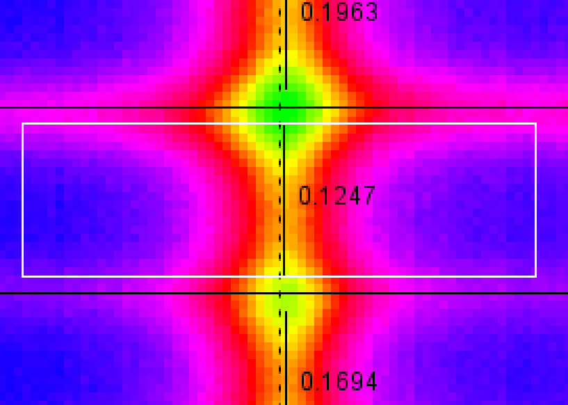
The box is centered horizontally around the expected leaf position (vertical dashed line) The vertical top and bottom of the box are 0.5 mm (a configurable value) from the measured leaf sides (horizontal solid lines). The 0.5 mm space isolates the measurement of this leaf end from the vertically adjacent leaf ends. Note that the vertical solid lines (the measured leaf ends) also show this 0.5 mm gap.
The average pixel value is found For each row of pixels in the box. All pixels that are above the average are processed to find their horizontal center of mass:
center of mass = (sum of value * position) / (number of pixels)
The center of masses of each pixel row are averaged to find the center of the leaf end. This value is then added to the collimator centering value, yielding the final result.
Some justifications for the algorithm:
Note that the edges of the bounding box will usually not be at pixel boundaries. To accommodate this, pixels that are only partially included in the box are weighted accordingly. For example, if a row of pixels is 40% inside the box, then the row would be given a 40% weight.